Executive Summary: 

• Policymakers have increased attention to current account deficits. Though experts debate whether current account deficits negatively impact the economy, many have also put forward theories regarding the influence of money supply on the current account. 

• The classic AA-DD model predicts that in the short term, an increase in money supply should result in a current account increase (in other words, a reduction of existing deficits). 

• However, regressions run on the broad money growth and current account as a percentage of GDP show little correlation between the two variables, highlighting the ineffectiveness of money supply as a tool to target the current account.  

As part of his rationale for increasing tariffs, President Trump has focused on the U.S.’s trade deficits. Experts have long debated whether trade deficits matter; some argue a trade deficit simply signals that the region is attractive to foreign investment and has strong consumer demand, while others have instead contended that a trade deficit could become worrisome if it is persistent and there comes a point when foreign investors are no longer willing to finance the deficit. This analysis does not seek to address whether a current account deficit is worrisome or not. Instead, it seeks to examine one potential avenue for impacting the current account: money supply.  

Several articles have previously examined the relationship between money supply and the current account balance. For example, experts from the Central Bank of the Republic of Turkey argue that periods of monetary tightening should see the foreign trade balance and current account positively impacted due to their impact on domestic demand. Other experts instead contend that an increase in money supply should place downward pressure on the trade deficit as an increase in money supply tends to depreciate the home currency.  

Theoretically, one should be able to see the relationship between money supply and the current account deficit using the AA-DD model, which incorporates both the impact of domestic demand and the exchange rate. The model defines the AA curve as the asset market, with an inverse correlation between exchange rates and output, or GDP. This inverse correlation arises from the assumption of interest parity. Note that interest parity does not actually hold in the short run, so this may be an unrealistic assumption. When output increases, there should be an increase in money demand. Given a constant money supply, this increases domestic interest rates. With foreign interest rates unchanged, the exchange rate must appreciate as otherwise there would be an opportunity for arbitrage.  

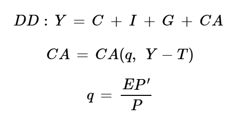
The model defines the DD curve as the goods market, with output defined as a function of consumption, C, investment, I, government spending, G, and the current account, CA. It further defines the current account as a function of relative prices, q, and disposable income, Y-T, where Y is output and T is tax level. Note that relative price is defined to be the exchange rate, E, times the ratio between foreign price level P’ and home price level P. When the exchange rate E increases, relative price q also increases. This means that it is relatively more expensive for the home country to import foreign goods, meaning imports fall, and it is cheaper for foreign countries to import the home country’s goods, meaning exports rise. As the current account is defined as exports minus imports, this means the current account increases, thus increasing output. Thus, the DD curve displays a positive relationship between E and Y.  

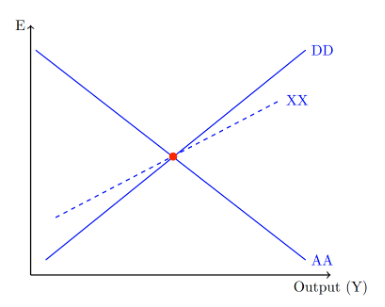
 Several useful equations for the model and a graphical representation are shown below. The graph below also shows a dotted line for the XX curve. The XX curve is used to show the current account balance directly; any point above the curve represents a surplus while any point below represents a deficit. Any point on the line represents a current account of 0, indicating that imports equal exports. 

Now, consider the short-term impact of a permanent increase in money supply using the above model. If our money supply increases, then given a constant money demand, domestic interest rates should decrease, and thus the home currency must depreciate assuming interest rate parity holds. Thus, as for every output level our exchange rate must be higher, the AA curve shifts outward. In the short term, there will be no shifts in the DD and the XX curve given that price levels have not yet had the time to adjust. The shifts in the curves are shown in the graph below. 

From the graph above, it is clear that the model predicts that a permanent increase in monetary supply increases the current account surplus in the short term as the orange equilibrium point is above the XX line. In the long term, the model predicts that the DD and XX curves will both shift upwards, returning the economy to equilibrium both in terms of output and current account, though the exchange rate will remain impacted.  

Notice that the graph above also assumes that a country begins with a balanced current account. This is an unrealistic assumption for most countries, but an increase in monetary supply will impact the current account of countries in the same way regardless of if they start in a balance. Thus, the model indeed predicts an increase in the current account in the short run regardless of its initial status. 

This analysis seeks to check the reliability of this model in predicting the short-term impact of an increase in money supply on a country’s current account deficit. To understand the overall relationship between money supply and the current account deficit, this analysis first runs a regression individually for each country so the relationship between money supply and current account for each individual country is clear (See Appendix). The regressions are then pooled afterwards so that the overall correlation is analyzed. This procedure is done twice to account for different potential “short runs”. First, the data uses the changes in broad money growth and current account as a percentage of GDP in the same year. The second treatment accounts for a one-year lag. 

The individual regressions will compute the values of B₀ and B₁ in the below equation. Essentially, the regression is calculating the line of best fit for the data, with B₀ as the y-intercept and B₁ as the slope. If B₁ is positive, then broad money growth and current account as a percentage of GDP are positively correlated, as the theoretical model predicts. On the other hand, if B₁ is negative, then the two are negatively correlated. A small B₁ indicates there may be little correlation between the two values.  

Regressions for Individual Countries, Same Year 

Data from the World Bank Group 

Regressions for Individual Countries, One Year Lag 

Data from the World Bank Group 

Notice that both tables above show a variety of positive and negative values of B₁ for countries. The values of B₁ also tend to be quite small, though they are slightly larger in the first data table with no lag. In the first chart, 6/20 countries have a negative coefficient for B₁, while in the second chart, 10/20 countries have negative coefficients. This shows there seems to be little correlation between broad money growth. 

The pooled regressions for the data are now examined. A pooled regression treats all the values in a data set equally and does not consider cross-country differences. This measure was chosen to see the overall pattern without controlling cross-country differences, as the individual regressions already give insight into individual relationships.  

Pooled Regression, Same Year 

Data from the World Bank Group 

Pooled Regression, One Year Lag 

Data from the World Bank Group 

The pooled regression for the same year gives B₁ as 0.0123. This means that for every 1% increase in broad money growth, there was a 0.0123% increase in current account as a percentage of GDP. While this is a positive value, as the theoretical model expects to find, the value is very small. With a calculated p-value of 0.614, the findings are also statistically insignificant. Thus, at least looking at data from the same year, there does not seem to be a strong correlation between the increase in money supply and the current account. 

The pooled regression for a one-year lag gives B₁ as -0.0252. This means that for every 1% increase in broad money growth, there was a 0.0252% decrease in current account as a percentage of GDP. With a calculated p-value of 0.381, this finding is still quite statistically insignificant. 

Overall, there seems to be no strong correlation between an increase in money supply and changes in the current account, despite the predictions given by the AA-DD model. This could be for a variety of reasons. For example, the AA-DD model assumes that interest parity holds, which is not supported by empirical data. Moreover, country-specific macroeconomic characteristics may also impact the relationship between money supply and current account deficit, such as the stability of an economy. Therefore, while the AA-DD model certainly captures the important theoretical relationship between money supply and current account, its predictions may not fully capture the effects seen in the real world. Policymakers should thus be sure to examine both theoretical models and empirical evidence when it comes to targeting the current account.   

Appendix:  

The regressions assess 20 countries of varying development levels.  To measure the change in money supply, the analysis uses the broad money growth data reported by countries to the World Bank. Though broad money growth is a more general measure of money supply than others typically used, such as M2, selecting this measure allows for more consistency across countries, especially those at different development levels. Next, the analysis also used both the current account balances and the GDPs of countries reported to the World Bank. First, the current account is calculated as a percentage of GDP for each year, and then the percentage change from year to year is calculated. This is done to account for cross-country and GDP variability.