Executive Summary

• An overheating economy, increased policy uncertainty, and decreased confidence have heightened recession risks for 2025.
• Recession modeling empowers policymakers to act early to mitigate the effects of economic downturns.
• This paper uses a weighted logit model to predict the probability of a recession within twelve months, predicting a 53 percent chance as of April 24, 2025. 

Introduction

Recession fears have arisen in early 2025, citing an overheating economy, high policy uncertainty, and decreased consumer confidence. Although inflation remains steady, the output gap (the difference between real and potential GDP) is signaling heating conditions that require policy correction. Michigan’s Survey of Consumers has decreased drastically while the Economic Policy Uncertainty Index is at its highest levels since the 2020 pandemic. Amid uncertainty, recession modeling gives policymakers the tools to assess data-driven recession probabilities. Binary logit models empower policymakers to choose appropriate action based off the predicted probability of a recession event. This paper employs one such model, finding that current data suggests the predicted probability of a U.S. recession within twelve months is 53 percent. The model suggests the yield curve remains a leading indicator, with the addition of the output gap significantly improving predictive power. This model outperforms traditional yield curve models by 12.3 percent in AUROC. 

Background and Literature Review

The National Bureau of Economic Research (NBER) produced the formal definition of a recession. NBER economists decided a recession is “a significant decline in activity spread across the economy, lasting more than a few months, visible in industrial production, employment, real income, and wholesale-retail trade” (Leamer, 2008). Quantitatively, the rule of thumb arrives at the consensus negative gross domestic product (GDP) growth for two consecutive quarters constitutes a recession. The problem with these definitions of a recession is that a country must be in, or past the period to formally recognize it as a recession. 

The benefit of recession modeling comes from using current economic conditions and comparing to historical recession periods. This is to give policymakers the ability to make decisions in an effort to mitigate or even avoid harsh downturns in the business cycle. Previous literature relies heavily on financial indicators, specifically the yield curve, at predicting recessions. Estrella and Mishkin (1996) use the yield curve, which is the interest rate on the ten-year Treasury note minus the three-month Treasury bill. Historically this has been an accurate indicator based off the properties of the curve. In the past when the curve has become inverted (negative), recessions have followed. An inverted curve means the rate on the ten-year note is decreasing, signaling worsening expectations of long-term conditions relative to the short term. The yield curve gives a simple method for evaluating recession risk. In recent years however, the yield curve has remained inverted with no near-term recession to follow. While beneficial against previous data, the yield curve gives false positives when applied to data from the past 3 years. 

Traditional models, like the one used in Liu and Moench (2014) add additional macroeconomic indicators and multiple lead periods to enhance predictive power. Combining leading hard data indicators along with the yield curve strengthens model performance at greater lead times. Liu and Moench also introduce the area under the receiver operating curve (AUROC) for model evaluation. The AUROC is used in binary classification, examining the tradeoff between the true positive rate and the false positive rate. Liu and Moench find their combination of indicators outperforms just the yield curve, with an AUROC of 0.94 compared to 0.83. This provides a strong tool for model selection and evaluation. 

More recent publications are increasingly using soft data to provide more insight. This soft data includes consumer expectations index and the economic policy uncertainty index. Chung (2022), and Baker, Bloom, and Davis (2016) highlight the importance of soft indicator selection on economic conditions. While Baker et al. does not focus on recession modeling, it does strengthen the case that consumer expectations influence macroeconomic indicators. 

The model employed in this paper draws strengths from each of the above. A weighted logit model is used to account for class imbalances. Financial indicators, macroeconomic indicators, and sentiment indexes are combined to maximize the predictive power of the model. Although more complex than the yield curve, the addition of new indicators provides meaningful insight into recession modeling. 

Data and Methodology

Seven core indicators have been included in the model: Consumer expenditure (transformed to monthly percent change; PCEPCT), the yield curve (T10Y3M), disposable income (DSPIC96), the S&P500 index (SP500), the economic policy uncertainty index (transformed to percent change from one year ago; EPU), the consumer sentiment index (transformed to percent change from one year ago; CSENT), and the output gap (OGAP). Linear interpolation is used to transform the output gap from quarterly to monthly observations. All data is sourced from the Federal Reserve Bank of St. Louis Economic Database (FRED). The data spans monthly, from January 1985 to March 2025. PCE is intended to capture consumer behavior in response to economic conditions. A slowdown in consumer expenditure may be an early warning sign for overall demand and economic overheating. The yield curve is the ten-year interest rate minus the three-month rate. Historically the yield curve has become negative before every major NBER recession. Disposable income is chosen to reflect personal financial health and control for wage growth. The S&P500 index reflects investor confidence. Changes in the level of the S&P500 indicates uncertainty in markets, therefore increasing recession risks. EPU is an indexed measure that captures attitude and certainty in economic policy. Baker et al. (2016) find increases in the EPU can lead to declines in investment, output, and employment. The output gap measures the relative temperature of the economy. Consumer sentiment is taken from the Michigan Survey of Consumers. It is an indexed soft data measure that captures general consumer attitude towards the economy. The output gap is the difference between actual and potential gross domestic product (GDP). Actual GDP over 1.5-2 percent of potential has been followed by a recession since 1990. The current Q3 2024 OGAP reading is measured at 1.86 percent. Recession dummy variables are generated with lead times of 3, 6, 9, and 12 months. Recessions identified in this model come from the NBER defined recessions. The dummy variables with increasing lead times are meant to determine the effect of each core variable on recession.

A weighted logit model is employed to predict the log-odds of a recession event. Log-odds are then transformed into probabilities for ease of interpretation. Recessions, while not rare, account for only 7.7 percent of the observations included in this study. Class imbalance risks are relevant because of the class sizes. To correct for class imbalances, a weighted model is estimated. The weight of each observation is defined as the inverse proportion of the class size. 

Let y_i denote the recession indicator where y_i = 1 indicates a recession. The weights w_i follow the form presented in Equation 1:

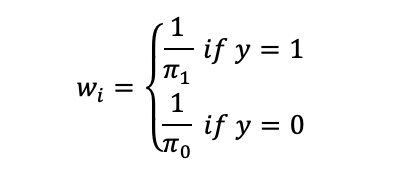
Where π₁ and π₀ represent the sample proportion of recessions and non-recessions. 

The log-odds model is defined in Equation 2 as: 

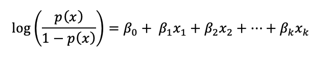
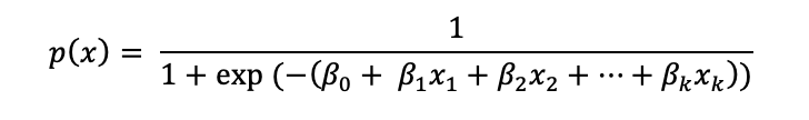
Where p(x) is the probability of a recession given variables x_i. The following probability prediction is given by Equation 3: 

The model parameters are found using maximum likelihood estimates, with the weighted log-likelihood function presented in Equation 4:

Where n denotes the total number of observations. 

The next section details robustness tests and model evaluation. 

Model Validation

The 12 month lead model is used in this study. This ensures a medium-term forecast while maintaining robust results. A lead time of 12 months allows time for policymakers to make data-driven decisions in a timely fashion to prevent downturns. Models using lead times of less than 12 months risk enacting reactive policy instead of proactive policy. 

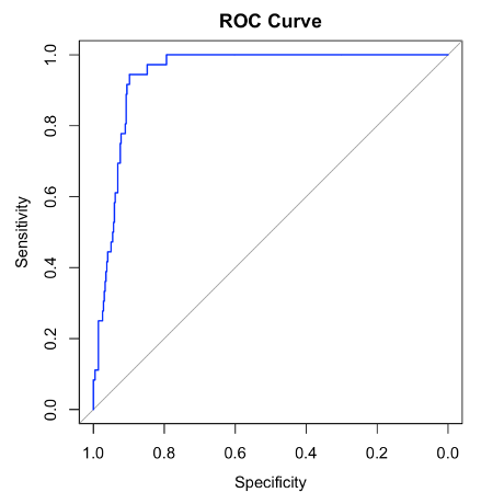
A ROC curve is developed to evaluate the model’s sensitivity vs specificity, or the true positive and false positive tradeoff. AUROC falls between 0 and 1, with an AUROC of 1 having perfect discriminatory power and 0.5 being equal to random guessing. ROC is used here instead of accuracy for two main reasons. Using accuracy as a measure of fit poorly estimates in cases of class imbalances. This is because if one selected “no recession” for every observation, they would be correct in 92.3 percent of cases from this sample. AUROC is threshold independent, and given the low frequency of recessions AUROC provides a more robust measure of fit compared to accuracy. The weighted logit model achieved an AUROC of 0.944, signifying excellent discriminatory power. As shown in Figure 1 below below displays the ROC curve and attributed AUROC. 
Figure 1:

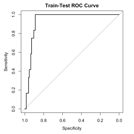
A train-test split was also employed to further validate the model’s performance. The model was re-estimated using a random sample of 70 percent of the total observations. The predicted probabilities were then assessed on the unseen 30 percent of data. An AUROC curve was generated from the test data to assess the model’s fit to unseen data. The corresponding AUROC in the test phase was 0.938, again signifying strong discriminatory power. Figure 2 shows the corresponding ROC curve and AUROC value. 

Figure 2:

In determining the optimal risk threshold, Youden’s J statistic was employed. Youden’s J is defined as the sum of sensitivity and specificity minus one. This statistic identifies the threshold that maximizes discriminatory power. Using this criterion the optimal threshold from the sample is 0.45. Observations with probabilities above 45 percent are labeled as high risk in the final model. 

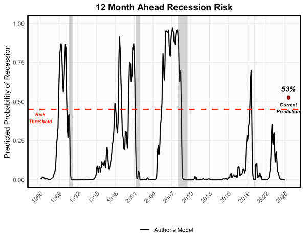
To further illustrate model fit, Figure 3 presents the historical predicted probabilities of a recession from January 1985 to February 2025. The graph shows NBER recessions in shaded regions and demonstrates the model’s ability to detect variability in recession indicators before a recession event occurs. 

Figure 3:

Regression Results

The weighted logistic regression gives the strict log-odds of the event. Log-odds gives the natural logarithm of the odds of an event occurring, with positive values indicating higher likelihood and negative values a lower likelihood. Table 1 shows the different models with staggered lead times to determine the relative importance of each key variable at different leads. The 12 month lead model 1)provides the most statistically significant results. The coefficient on PCEPCT suggests an increase in one unit of expenditure is predicted to increase the log-odds of a recession by 2.352 units. Increasing the yield curve (T10Y3M) by unit is predicted to decrease the log-odds of a recession by 1.832 units. Increasing disposable income by one unit is predicted to increase the log-odds of a recession by 0.001 units. An increase of the S&P500 by one unit is predicted to decrease the log-odds of a recession by 0.004 units. An increase in consumer sentiment by one unit is predicted to decrease the log-odds of a recession by 0.080 units. Increasing the EPU by one unit is predicted to increase the log-odds of a recession by 0.009 units. Increasing the output gap by one unit is predicted to increase the log-odds of a recession by 1.706 units. Each of the variables is intended to be interpreted holding all else constant. 

Table 1:

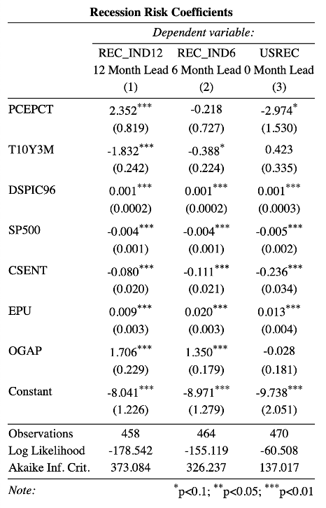
The key components driving the model are consumer expenditure, the yield curve, and the output gap. Consumer expenditure holds a positive value, which is contrary to initial economic intuition. This could be attributed to the overheating economy. With 12 months lead, demand is still likely high and effects from overconsumption and inflation have likely not taken place. This rationale is further supported by the coefficients at 6 months and 0 months. While the 6-month coefficient is not statistically significant, the 0 month coefficient is, and its sign is reversed from the 12 month model. The sign reversal signifies the change in consumption habits in economic downturns. Already the data show expenditure slowing down, which could hint at a recession already looming. At 12 months lead the economy is nearing its peak heating conditions, contributing to expenditure increasing the log-odds of a recession inside 12 months. The yield curve has historically been a strong indicator of recessions at the 12-month lead time. The coefficient on the yield curve supports the notion that an inverted yield curve increases the risk of a recession. The coefficient on the output gap also follows economic intuition of a heating economy. Pushing the economy past potential GDP creates an inflationary environment prone to downturns. 

Table 2 depicts the current level for all variables:

Change Expenditure (%)	Yield Curve	Disposable Income	S&P500	EPU	Output Gap	Consumer Sentiment
0.43%	-0.06	17756.2	5373.58	369.5	1.86%	-25.9

Given the data available, the model estimate predicted probability of a recession in 12 months is 53 percent. 

The next section discusses the policy tools available when in high-risk recession periods and the current challenges policymaking organizations have in addressing recession concerns. 

Policy Implications and Concluding Remarks

When Probabilities Exceed the Threshold

Policymakers are equipped with the proper tools to respond to changing economic conditions. Monetary policy actions are actions central banks can take to influence macroeconomic conditions. In response to recession fears, a key monetary policy tool is revising interest rates. Cutting interest rates stimulate demand if facing economic downturns. Lowering interest rates stimulates demand, increasing consumer and investor activity in the economy. This approach is typically taken to keep growth at the Federal Reserve (Fed) projected two percent growth. The U.S. economy is showing heating however, with some signs already pointing to cooling. Previously when dealing with an overheating economy the Fed has raised rates too sharply leading to a severe economic downturn. This is evident with the dotcom bubble and 2008 recession. The Fed has a tight rope to walk when combatting a heating economy. Historically a sit and wait for data institution may cause rates to change too late for fears of instigating another hard landing. 

The federal government possesses fiscal policy powers. Fiscal policy is the use of government spending and taxation to influence the economy. Expansionary fiscal policy would include cutting taxes to stimulate demand. This approach can be more tailored and target certain industries to promote economic activity. Industry targeted tax cuts like the Investment Tax Credit (ITC) were used in the 60s and 70s to promote investment in capital intensive industries and were received with relative success. Cutting taxes for individuals can also limit the probability of a recession. Tax cuts of this nature increase disposable income and hopefully increase consumer expenditure to strengthen a weakening economy. Broader, across the board tax cuts like Reagan’s 1981 Economic Recovery Tax Act support this action as well. 

Certainty also plays a large role in countering economic downturns. Providing targeted approach from both a fiscal and monetary policy relays a sense of confidence and direction towards consumers and investors. Uncertain conditions give rise to low consumer confidence, which is linked to consumer expenditure. Uncertainty also decreases confidence in the stock market, which is a major gauge of investor sentiment. By acknowledging and providing a certain direction, policymaking organizations can increase confidence in markets. 

Current Policy Challenges

Current policy actor’s communication so far has downplayed the negative impact of its economic policy initiatives regarding tariffs. The bipartisan and academic consensus on the impact of tariffs creates a head-to-head battle between fiscal and monetary policy directives. This policymaker tug-of-war has already been bad for markets and consumer confidence, with the S&P500 and consumer sentiment dropping to their lowest levels since the pandemic. 

With their dual mandate to combat inflation and maintain full employment, the Fed has a multitude of complex considerations to review. A heating economy, inflation from tariff policy, and no unified front coming from Federal policymakers is causing decision making to be even more difficult. This scenario makes traditional policymaking tools to less effective. Cutting rate too early and the impact of tariffs might cause inflation to spiral out of control. Cutting them too late will limit their effectiveness. There is also a scenario where the Fed might delay rate increases in response to inflation from tariff policy. As seen in the past increasing rates too sharply has the potential for another hard landing, especially since the costs associated with tariffs are typically passed to the consumer. Lowering interest rates would also stimulate demand and increase the output gap, however in an already overheating economy this could also risk worsening inflationary pressures. 

The Fed is likely to wait in making a decision until more data comes in. This will ensure they can determine how far each mandate is from their target and tackle the one furthest from target. The expected economic impact of tariff policies is likely to be severe. The United States and global supply chain are more connected than ever because of comparative advantage. Disruption of global supply chains to America has high potential to be drastic and the data show recession odds are increasing. The Fed is likely to cut rates in Q3 2025 based on the hard data received from Q2. Final Q1 2025 estimates will likely show modest front-loading in demand in anticipation of future higher prices via tariffs, and if Q2 data confirms contractions it has potential to warrant rate cuts. 

The model estimate current prediction of a recession inside the next 12 months sits at 53 percent. This is above the threshold specified for high risk, and policymakers should look to act soon. The model provided is robust and provides a data-driven approach to calculating the risk of a recession.